IMDB Data Analysis

Loading the data
movies <- read_csv(here::here("data", "movies.csv"))
glimpse(movies)
## Rows: 2,961
## Columns: 11
## $ title <chr> "Avatar", "Titanic", "Jurassic World", "The Avenge…
## $ genre <chr> "Action", "Drama", "Action", "Action", "Action", "…
## $ director <chr> "James Cameron", "James Cameron", "Colin Trevorrow…
## $ year <dbl> 2009, 1997, 2015, 2012, 2008, 1999, 1977, 2015, 20…
## $ duration <dbl> 178, 194, 124, 173, 152, 136, 125, 141, 164, 93, 1…
## $ gross <dbl> 7.61e+08, 6.59e+08, 6.52e+08, 6.23e+08, 5.33e+08, …
## $ budget <dbl> 2.37e+08, 2.00e+08, 1.50e+08, 2.20e+08, 1.85e+08, …
## $ cast_facebook_likes <dbl> 4834, 45223, 8458, 87697, 57802, 37723, 13485, 920…
## $ votes <dbl> 886204, 793059, 418214, 995415, 1676169, 534658, 9…
## $ reviews <dbl> 3777, 2843, 1934, 2425, 5312, 3917, 1752, 1752, 35…
## $ rating <dbl> 7.9, 7.7, 7.0, 8.1, 9.0, 6.5, 8.7, 7.5, 8.5, 7.2, …Count of movies by genre, ranked in descending order
movies %>%
  group_by(genre) %>%
  summarise(count_genre = count(genre)) %>%
  arrange(desc(count_genre))
## # A tibble: 17 × 2
## genre count_genre
## <chr> <int>
## 1 Comedy 848
## 2 Action 738
## 3 Drama 498
## 4 Adventure 288
## 5 Crime 202
## 6 Biography 135
## 7 Horror 131
## 8 Animation 35
## 9 Fantasy 28
## 10 Documentary 25
## 11 Mystery 16
## 12 Sci-Fi 7
## 13 Family 3
## 14 Musical 2
## 15 Romance 2
## 16 Western 2
## 17 Thriller 1Average gross earning and budget (gross and budget) by genre
movies %>%
  group_by(genre) %>%
  summarise(mean_gross = mean(gross), mean_budget = mean(budget)) %>%
  mutate(return_on_budget = mean_gross/mean_budget) %>%
  arrange(desc(return_on_budget))
## # A tibble: 17 × 4
## genre mean_gross mean_budget return_on_budget
## <chr> <dbl> <dbl> <dbl>
## 1 Musical 92084000 3189500 28.9
## 2 Family 149160478. 14833333. 10.1
## 3 Western 20821884 3465000 6.01
## 4 Documentary 17353973. 5887852. 2.95
## 5 Horror 37713738. 13504916. 2.79
## 6 Fantasy 42408841. 17582143. 2.41
## 7 Comedy 42630552. 24446319. 1.74
## 8 Mystery 67533021. 39218750 1.72
## 9 Animation 98433792. 61701429. 1.60
## 10 Biography 45201805. 28543696. 1.58
## 11 Adventure 95794257. 66290069. 1.45
## 12 Drama 37465371. 26242933. 1.43
## 13 Crime 37502397. 26596169. 1.41
## 14 Romance 31264848. 25107500 1.25
## 15 Action 86583860. 71354888. 1.21
## 16 Sci-Fi 29788371. 27607143. 1.08
## 17 Thriller 2468 300000 0.00823Top 15 directors who have created the highest gross revenue in the box office
movies %>%
  group_by(director) %>%
  summarise(total_gross = sum(gross),
            mean_gross = mean(gross),
            med_gross = median(gross),
            sd_gross = sd(gross)) %>%
  slice_max(total_gross, n=15)
## # A tibble: 15 × 5
## director total_gross mean_gross med_gross sd_gross
## <chr> <dbl> <dbl> <dbl> <dbl>
## 1 Steven Spielberg 4014061704 174524422. 164435221 101421051.
## 2 Michael Bay 2231242537 171634041. 138396624 127161579.
## 3 Tim Burton 2071275480 129454718. 76519172 108726924.
## 4 Sam Raimi 2014600898 201460090. 234903076 162126632.
## 5 James Cameron 1909725910 318287652. 175562880. 309171337.
## 6 Christopher Nolan 1813227576 226653447 196667606. 187224133.
## 7 George Lucas 1741418480 348283696 380262555 146193880.
## 8 Robert Zemeckis 1619309108 124562239. 100853835 91300279.
## 9 Clint Eastwood 1378321100 72543216. 46700000 75487408.
## 10 Francis Lawrence 1358501971 271700394. 281666058 135437020.
## 11 Ron Howard 1335988092 111332341 101587923 81933761.
## 12 Gore Verbinski 1329600995 189942999. 123207194 154473822.
## 13 Andrew Adamson 1137446920 284361730 279680930. 120895765.
## 14 Shawn Levy 1129750988 102704635. 85463309 65484773.
## 15 Ridley Scott 1128857598 80632686. 47775715 68812285.Ratings by genre.
# TABLE WITH SUMMARY STATISTICS
movies %>%
  group_by(genre) %>%
  summarise(mean_rating  = mean(rating),
            min_rating   = min(rating),
            max_rating   = max(rating),
            med_rating   = median(rating),
            sd_rating    = sd(rating))
## # A tibble: 17 × 6
## genre mean_rating min_rating max_rating med_rating sd_rating
## <chr> <dbl> <dbl> <dbl> <dbl> <dbl>
## 1 Action 6.23 2.1 9 6.3 1.03
## 2 Adventure 6.51 2.3 8.6 6.6 1.09
## 3 Animation 6.65 4.5 8 6.9 0.968
## 4 Biography 7.11 4.5 8.9 7.2 0.760
## 5 Comedy 6.11 1.9 8.8 6.2 1.02
## 6 Crime 6.92 4.8 9.3 6.9 0.849
## 7 Documentary 6.66 1.6 8.5 7.4 1.77
## 8 Drama 6.73 2.1 8.8 6.8 0.917
## 9 Family 6.5 5.7 7.9 5.9 1.22
## 10 Fantasy 6.15 4.3 7.9 6.45 0.959
## 11 Horror 5.83 3.6 8.5 5.9 1.01
## 12 Musical 6.75 6.3 7.2 6.75 0.636
## 13 Mystery 6.86 4.6 8.5 6.9 0.882
## 14 Romance 6.65 6.2 7.1 6.65 0.636
## 15 Sci-Fi 6.66 5 8.2 6.4 1.09
## 16 Thriller 4.8 4.8 4.8 4.8 NA
## 17 Western 5.7 4.1 7.3 5.7 2.26movies %>%
ggplot(aes(x = rating, color = genre, fill = genre)) +
geom_density(size=1, alpha = .1) +
theme_minimal() +
facet_wrap(~genre) +
labs(
title="Ratings density by Genre",
subtitle="IMDB Movies Dataset",
caption = "Source: Kaggle IMDB 5000 movie dataset",
x="Rating",
y="% Density"
) +
theme(legend.position = "none")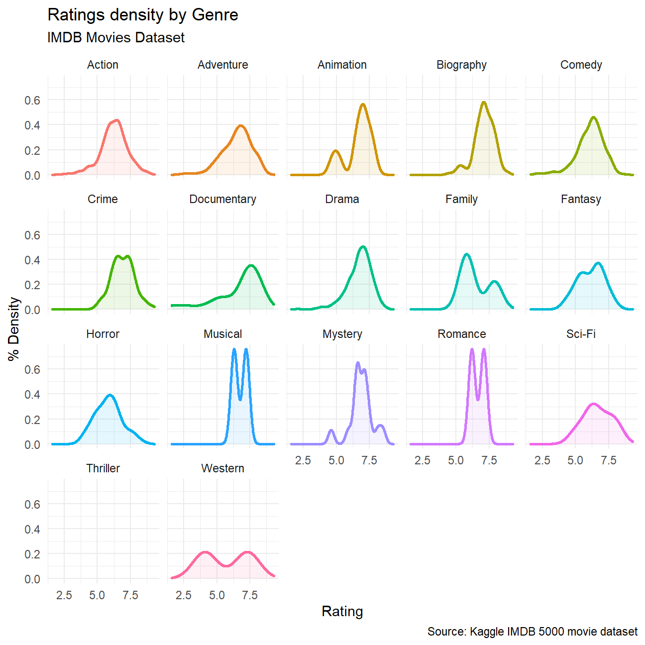
Confidence interval for mean ratings between Spielberg and Burton
 confidence_interval <- movies %>%
  filter(director == 'Steven Spielberg' | director=='Tim Burton') %>%
  group_by(director) %>%
  summarize(mean_rating = mean(rating),
            sd_rating = sd(rating),
            count=n(),
            t_critical = qt(0.975, count-1),
            se_rating = sd(rating)/sqrt(count),
            margin_of_error = t_critical * se_rating,
            rating_high = mean_rating + margin_of_error,
            rating_low = mean_rating - margin_of_error)

points <- confidence_interval %>%
  select(c('director', 'mean_rating','rating_high','rating_low'))

ggplot(confidence_interval, aes(x=mean_rating, y=director)) +

  geom_rect(aes(xmin = 7.27, xmax = 7.33, ymin = -Inf, ymax = Inf), fill="light gray") +

  geom_errorbar(aes(xmin=rating_low, xmax=rating_high, colour=director), width=.2,
                 position=position_dodge(.9)) +

  geom_point(data=points, aes(x=mean_rating, y=director)) +
  geom_text(aes(label=round(mean_rating, digits=2)), nudge_y=0.04, size=3) +

  geom_point(data=points, aes(x=rating_high, y=director)) +
  geom_text(aes(label=round(rating_high, digits=2)), nudge_x=0.35, nudge_y=0.04, size=3) +

  geom_point(data=points, aes(x=rating_low, y=director)) +
  geom_text(aes(label=round(rating_low, digits=2)), nudge_x=-0.35, nudge_y=0.04, size=3) +

  labs(title="Do Spielberg and Burton have the same mean IMDB ratings?", subtitle="95% confidence intervals overlap", x="Mean IMDB Rating", y="") +
  theme(legend.position = 'none') +

  NULL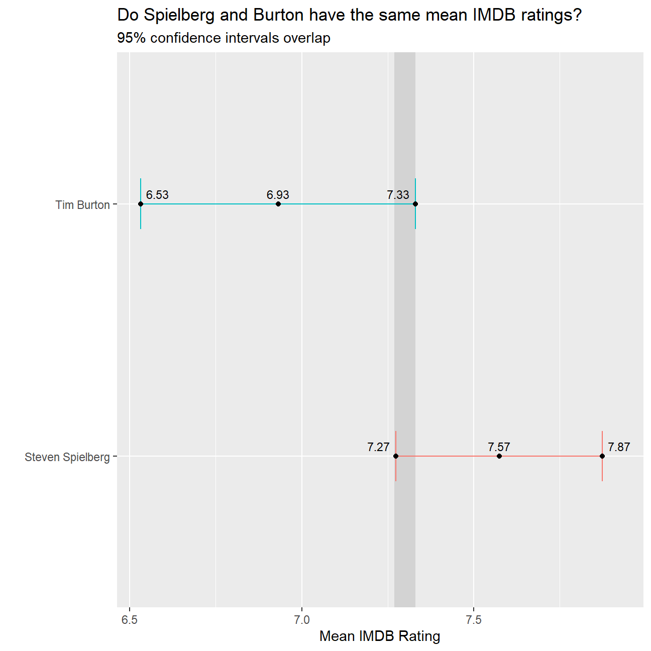
T-Test for mean ratings using t_test
t_data <- movies %>%
                 filter(director == 'Steven Spielberg' | director=='Tim Burton')
t.test(rating~director, t_data)
##
## Welch Two Sample t-test
##
## data: rating by director
## t = 3, df = 31, p-value = 0.01
## alternative hypothesis: true difference in means between group Steven Spielberg and group Tim Burton is not equal to 0
## 95 percent confidence interval:
## 0.16 1.13
## sample estimates:
## mean in group Steven Spielberg mean in group Tim Burton
## 7.57 6.93T-test for mean ratings using infer
# calculating observed statistic
obs <- movies %>%
  filter(director == 'Steven Spielberg' | director=='Tim Burton') %>%
  specify(rating ~ director) %>%
  calculate(stat = "diff in means")

# simulate data
set.seed(4567)
sim <- movies %>%
  filter(director == 'Steven Spielberg' | director=='Tim Burton') %>%
  specify(rating ~ director) %>%
  hypothesize(null = "independence") %>%
  generate(reps=1000, type='permute') %>%
  calculate(stat="diff in means")


visualize(sim) +
  shade_p_value(obs_stat = obs, direction = "greater")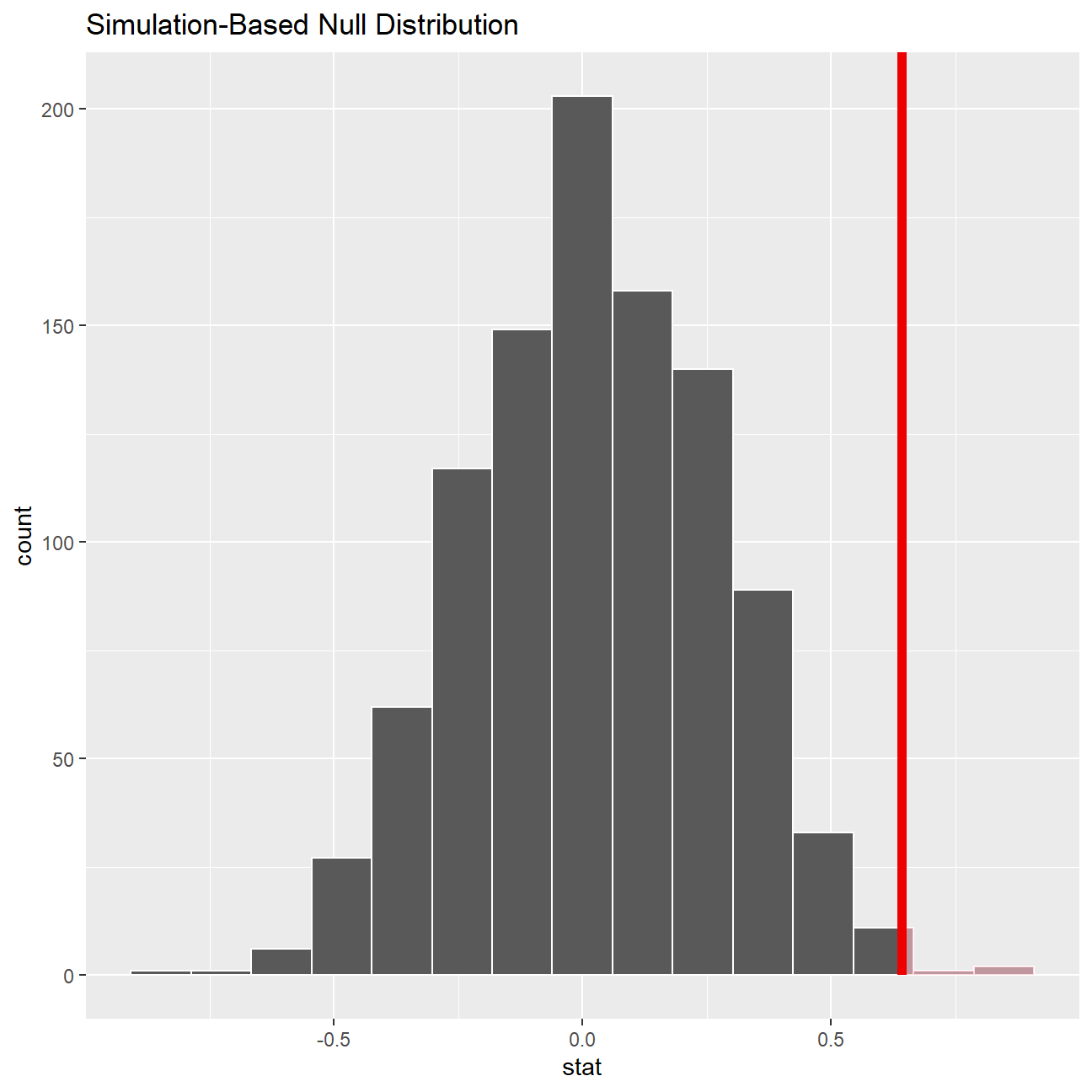
sim %>%
  get_p_value(obs_stat = obs, direction = "greater")
## # A tibble: 1 × 1
## p_value
## <dbl>
## 1 0.005